An Ode to Asymptotic Notations

August 26, 2017 ∙ 📖 12 min

On the La La Land of algorithms, there are ample ways to depict the efficiency and scalability of an algorithm especially when the input size is large. Altogether, these ways are called as Asymptotic Notations(Asymptotic Analysis). In this post, we’ll acquaint ourselves with these notations and we’ll see how we can leverage them to analyse an algorithm.

Note: I am writing this post in order to learn cause I strongly believe in learning by teaching. In case, you have suggestion/correction, please feel free to post in comment section.

Before we delve into the analysis of an algorithm, we need to know what’s an algorithm and why studying/analysing algorithms is important. So let’s get started.

What is an algorithm?

According to Merraim Webster,

An algorithm is a procedure for solving a mathematical problem (as of finding the greatest common divisor) in a finite number of steps that frequently involves repetition of an operation; broadly : a step-by-step procedure for solving a problem or accomplishing some end especially by a computer.

In other words an algorithm is simply a finite set of well-defined instructions, written to solve a specific problem (Ted-Ed: What’s an algorithm?). e.g. We want to find an element in an array. One way to find it, we traverse each element in the array and compare with the key element. If it’s equal then we say that element is present in the array else we continue traversing till the end of the array (Linear Search).

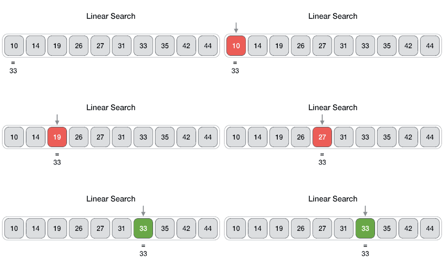
Generally, algorithms are written in the pseudo code. Pseudo code is simply the text written in an informal language which explains the algorithm and can be translated in any programming language. Think of pseudo code as a text-based algorithmic design tool. Let’s write pseudo code for the example above.

Algorithm:
Find Element(array, key)
a) Set i = 1;
b) if i is greater than array_size then go to step g.
c) if array[i] is equal to key then go to step f.
d) set i = i + 1;(increase i by 1).
e) go to step b.
f) print 'Present' and go to step h.
g) print 'Not present'.
h) Exit.
Pseudo Code:
findElement(array, key)
    for each item in array
        if item == key
            return 'Present'.
    return 'Not present'.

Here’s another algorithm which might be helpful for you if you are living alone.

According to Cormen’s Introduction to Algorithm,

An algorithm is said to be correct if, for every input instance, it halts with the correct output.

We supply various instances of input (including edge cases) to an algorithm to measure its correctness. For example, how linear search algorithm will behave if we pass an empty array as input.

Algorithms are unambiguous in nature.

It means that for an algorithm, each of its steps & inputs/outputs must be clear and lead to only one meaning.

Why Studying Algorithms?

As engineers, we always strive to provide better solutions. We know that often there are many ways to solve a problem and each way has its own strengths and weaknesses. Studying solutions/algorithms helps us to decide which solution to pick. For example to find an element in an array, instead of Linear Search we can use Binary Search if we know that our input array is sorted. While studying an algorithm we consider following questions:

1. Does it solve the problem with all possible inputs?
2. Does it use resources efficiently?
3. Can it be optimised?
4. Is it scalable?
5. Is there any better algorithm?
6. and the list goes on…

Execution of an algorithm requires many resources like computational time, memory, communication bandwidth, computer hardware etc. When we analyse an algorithm, we primarily focus on computational/running time and memory/space required for the algorithm (aka Time Complexity & Space Complexity). Let’s determine the time complexity of our Linear Search algorithm. Here’s a simple JavaScript program for LinearSearch.

Copy
/**
 * Linear Search.
 * @param array
 * @param element
 */
const linearSearch = (array, element) => {
  // Traverse elements of the array and compare
  // them
  for (let i = 0; i < array.length; i++) {
    // Compare element at ith position with
    // key element. If both are equal then return
    // the index.
    if (array[i] === element) {
      return i;
    }
  }
  // no element found. Returns -1.
  return -1;
};

You can see that our linearSearch function takes two parameters: array and element we wish to find. It simply traverses the array using for loop and compares every item of the array with element parameter. Let’s assume comparison statement takes time a unit of computer time and the size of array is n then

1. Best Case: First entry in the array is equal to element. Only one iteration, so time = a; (minimum time required to find the element).

2. Worst Case: Last entry in the array is equal to element Or Element not present in the array. n iterations, so time = a \* n; (maximum time required to find the element).

3. Average Case: Any entry between first and last matches to element. so required time will be between min and max time (a ≤ time ≤ a \* n).

By looking at above scenarios, we can conclude that the running time of an algorithm depends on the size of the input and the time taken by the computer to run the lines of code of the algorithm. In other words, we can think of running time as a function of the size of its input. eg. For Linear Search, it is F(n) = an.

Another important thing which we consider for analysis is the rate of growth of the function. The rate of growth(aka Order of Growth) describes how the running time increases when the size of input increases. Here’s the plot of running time for Linear Search with respect to input size.

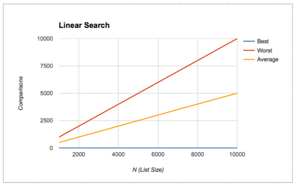
When we talk about the rate of growth, we mainly focus on the part of our function which has high impedance and causes drastic changes in the running time of algorithm especially when the input size is very large.

Consider a quadratic function F(n) = an² + bn + c. For very large value of n, term (bn + c) becomes less significant and the addition of it to an² barely make any difference. It’s like throwing a bucket filled with water in the ocean or on Big Show 😀. So we can knock it off. Now we are left with an².

As we know that a is constant coefficient and we want our entire focus to be on the size of input so we can knock off a as well. Consequently, we are left with n² and that’s what indeed matter for us. It tells us that running time of our function grows as n² which means that it’s growth rate is quadratic. Similarly, we can say that growth rate for Linear Search is linear (n).

When we remove the less significant terms and coefficients, we get the rate of growth of our function but we need more formal/generic way of describing them, that’s when we use asymptotic notations.

Think of asymptotic notations, as a formal way to speak about functions and classifying them.

Asymptotic notations has following classes or notations for describing functions:

1. O-Notation (Big Oh).
2. 𝛺-Notation (Big Omega).
3. ϴ-Notation (Theta).
4. o-Notation (Little Oh).
5. 𝜔-Notation (Little Omega).

In this post, we will discuss top 3 notations i.e. O, 𝛺 and ϴ. If you wish to read about other two notations, you can read them in CLRS. So let’s disucss them one by one.

O-Notation:

In plain English, Big oh notation is a way of estimating upper bound/limit of a function when the input is very large. Let’s write it in mathematical form.

O(g(n)) = {
    f(n): there exist positive constants c and k such that
    0 ≤ f(n) ≤ cg(n) for all n ≥ k
}

Don’t worry if you are not able to understand it. I am with you and “May the force be with us”. Let me break it down for you. At first, we have chosen an arbitrary constant called k as a benchmark for large input means our input is considered large only when n ≥ k. After that, we are defining the upper bound for our function f(n) with the help of function g(n) and constant c. It means that our function f(n)’s value will always be less than or equal to c * g(n) where g(n) can be any non-negative function for all sufficiently large n. For example, for Linear Search g(n) = n. So Time Complexity of Linear Search, for both worst case and average case, is O(n) i.e. Order of n. Time Complexity of Linear Search for best case is O(1) i.e. constant time (key element is the first item of the array).

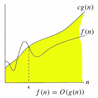
Big Oh notation is the most widely used notation for time complexity cause it talks about the upper bound of an algorithm which helps us to decide which algorithm is better. eg. algorithm of complexity O(n) will do better than algorithm of complexity O(n²) for sufficiently large input(it may not be true when input is small).

𝛺-Notation:

Omega notation is converse of Big Oh notation. It is a way of estimating lower bound/limit of a function when the input is significantly large.

Ω (g(n)) = {
    f(n): there exist positive constants c and k such that
    0 ≤ cg(n) ≤ f(n) for all n ≥ k
}

As we can see, the value of function is always greater than or equal to lower bound i.e. c * g(n).

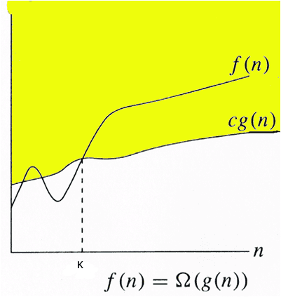
Omega notation is mainly useful when we are interested in the least amount of time required for the function/algorithm which make it the least used notation among other notations.

ϴ-Notation:

Theta notation is asymptotically tight bound, it means our function lies between upper bound and lower bound.

Θ(g(n)) = {
    f(n): there exist positive constants a, band k such that
    0 ≤ b * g(n) ≤ f(n) ≤ a * g(n) for all n ≥ k
}

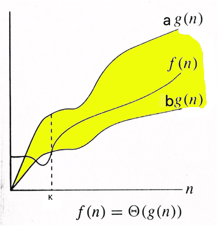
As we can see, if f(n) is theta of g(n) then f(n) always lies between b * g(n) and a * g(n) for all values of n which are greater than or equal to k. eg. we know that upper bound for Insertion Sort is order of n² (when array is sorted in reverse order, worst case) and lower bound is order of n (when array is already sorted, best case). So in ϴ notation we describe the time complexity for insertion sort using following statements:

1. Worst case time complexity of insertion sort is ϴ(n²).
2. Best case time complexity of insertion sort is ϴ(n).
3. Average case time complexity of insertion sort is ϴ(n²).

Which notation to use?

Often people ask which notation shall we use to describe the complexity of an algorithm? Well, it depends on the situation and the desired statement. Let’s take an example of Insertion Sort. We know that for Insertion Sort the worst case time complexity is ϴ(n²) and best case time complexity is ϴ(n). Can we say that the time complexity of insertion sort is ϴ(n²)? No. We can’t cause we know that for the best case it is ϴ(n). Similarly, we can not say that it’s ϴ(n) cause for the worst case it is ϴ(n²). An astute reader might ask, is there any way to make a single/blanket statement which covers both cases and tells us about the complexity instead of talking about the best case and the worst case? Yes. There is. What if in lieu of ϴ notation, we use Big O notation, then we can say that the time complexity of insertion sort is Order of n² i.e. O(n²) then we don’t need to worry about linear time i.e. O(n) cause upper bound n² covers it. A details discussion about which notation to use can be found on this StackExchange thread.

Summary

To summarise, we can say that asymptotic notations are fancy ways/classes of speaking about algorithms. They help us to compare one algorithm with another. They also help us to reason about our algorithms with various cases like best case, worst case, and average case.

References:

1. Introduction to Algorithm by CLRS.
2. Asymptotic Notations by GeeksForGeeks.
3. Khan Acadamy.
4. and of course Stackoverflow.

Hi, I am Hitesh.

|

• ← Salient Notes from “The Monk Who Sold His FERRARI”
• Binging Binary Search 🔎 →